기본적으로 아래처럼 한다.
cname <- c("x1", "x2", "x3","x4", "x5", "x6", "y")
german = read.table("c:\\data\\german1.txt", col.names = cname)
options(contrasts = c("contr.treatment", "contr.poly"))
german.object <- glm(y~.,family=binomial, data=german)
summary(german.object)
p <- predict(german.object, german, type="response")
german <- cbind(german, p)
head(german)
p는 y=1일 확률이다. 교제에서는 y=1이 불량고객이다.
> head(german)
   x1 x2  x3 x4 x5 x6 y          p
1 A11  6 A34  4 67  1 0 0.18170622
2 A12 48 A32  2 22  1 1 0.63312134
3 A14 12 A34  3 49  2 0 0.04812842
4 A11 42 A32  4 45  2 0 0.64393801
5 A11 24 A33  4 53  2 1 0.47102819
6 A14 36 A32  4 35  2 0 0.20127115
4 변수선택법 #
전진선택, 변수소거, 둘다
cname <- c("x1", "x2", "x3","x4", "x5", "x6", "y")
german = read.table("c:\\data\\german1.txt", col.names = cname)
#상수항만 포함한 초기모형
g.object <- glm(y~1, family=binomial, data=german)
#전진선택법
s.list <- list(upper = update(g.object, ~. +x1+x2+x3+x4+x5+x6))
step(g.object, scope=s.list, direction="forward")
#변수소거법
#s.list <- list(lower = update(g.object, ~. -x1-x2-x3-x4-x5-x6))
#step(g.object, scope=s.list, direction="backward")
#둘다
#s.list <- list(upper = update(g.object, ~. +x1+x2+x3+x4+x5+x6), lower = update(g.object, ~. -x1-x2-x3-x4-x5-x6))
#step(g.object, scope=s.list, direction="both")
결과
> step(g.object, scope=s.list, direction="forward")
Start:  AIC=1223.73
y ~ 1

       Df Deviance    AIC
+ x1    3   1090.4 1098.4
+ x3    4   1161.3 1171.3
+ x2    1   1177.1 1181.1
+ x5    1   1213.1 1217.1
<none>      1221.7 1223.7
+ x6    1   1221.7 1225.7
+ x4    1   1221.7 1225.7

Step:  AIC=1098.39
y ~ x1

       Df Deviance    AIC
+ x2    1   1051.9 1061.9
+ x3    4   1053.2 1069.2
+ x5    1   1085.0 1095.0
<none>      1090.4 1098.4
+ x4    1   1090.2 1100.2
+ x6    1   1090.3 1100.3

Step:  AIC=1061.9
y ~ x1 + x2

       Df Deviance    AIC
+ x3    4   1022.6 1040.6
+ x5    1   1046.7 1058.7
<none>      1051.9 1061.9
+ x4    1   1051.5 1063.5
+ x6    1   1051.9 1063.9

Step:  AIC=1040.58
y ~ x1 + x2 + x3

       Df Deviance    AIC
+ x5    1   1019.3 1039.3
<none>      1022.6 1040.6
+ x6    1   1022.5 1042.5
+ x4    1   1022.5 1042.5

Step:  AIC=1039.27
y ~ x1 + x2 + x3 + x5

       Df Deviance    AIC
<none>      1019.3 1039.3
+ x4    1   1019.2 1041.2
+ x6    1   1019.3 1041.3

Call:  glm(formula = y ~ x1 + x2 + x3 + x5, family = binomial, data = german)

Coefficients:
(Intercept)        x1A12        x1A13        x1A14           x2
    0.66510     -0.53186     -1.07608     -1.89880      0.03434
      x3A31        x3A32        x3A33        x3A34           x5
   -0.09915     -0.94696     -0.93433     -1.52607     -0.01277

Degrees of Freedom: 999 Total (i.e. Null);  990 Residual
Null Deviance:	    1222
Residual Deviance: 1019 	AIC: 1039
>
최종적으로 glm(formula = y ~ x1 + x2 + x3 + x5, family = binomial, data = german) 가 선택되었다. AIC가 가장 적은 모델이 선택된다.
참고: AIC (
![[http]](/moniwiki/imgs/http.png) 출처(http://blog.naver.com/pinokio129?Redirect=Log&logNo=80018702687)
출처(http://blog.naver.com/pinokio129?Redirect=Log&logNo=80018702687))
AIC 통계량

최적 모형을 결정하는 경우 모형의 설명능력과 모형의 절약성을 고려해야 함.
모형의 설명능력은 우도(likelihood)로서 측정될 수 있으며,
모형의 절약성은 복잡한 모형 보다는 간결한 모형이 선호되어야 한다는 것으로
추정 계수의 數가 많은 것에 대해 벌칙을 가함으로써 고려될 수 있다.
그러나 모형의 설명력과 절약성은 상충되는(trade-off)기준으로서,
왕왕 복잡한 모형이 설명력이 큰것을 발견 할 수 있다.
따라서 두 판단기준을 함께 고려한 선택규준이 필요하게 된다.
그것이 바로 정보기준 접근법으로 Akailke에 의하여 개발된
Akaike Information Criterion(AIC)이다.


   AIC = -2 log L +2n


여기서 'n': 파라미터 수를 나타내며, 'log L'은 대수우도(log-likelihood).
※ Akailke에 의하면 AIC통계량의 값이 최소가 되는 모형을 채택하여야 된다
D(Deviance)는 일반화된 선형 모형에서 모형의 적합도 검증 통량이다.
cname <- c("x1", "x2", "x3","x4", "x5", "x6", "y")
german = read.table("c:\\data\\german1.txt", col.names = cname)
options(contrasts = c("contr.treatment", "contr.poly"))
german.object <- glm(formula = y ~ x1 + x2 + x3 + x5, family = binomial, data = german)
summary(german.object)
결과
Call:
glm(formula = y ~ x1 + x2 + x3 + x5, family = binomial, data = german)

Deviance Residuals:
    Min       1Q   Median       3Q      Max
-1.7997  -0.8007  -0.4747   0.9283   2.4241

Coefficients:
             Estimate Std. Error z value Pr(>|z|)
(Intercept)  0.665099   0.476311   1.396 0.162607
x1A12       -0.531864   0.185402  -2.869 0.004121 **
x1A13       -1.076082   0.336956  -3.194 0.001405 **
x1A14       -1.898800   0.206314  -9.203  < 2e-16 ***
x2           0.034342   0.006329   5.426 5.76e-08 ***
x3A31       -0.099153   0.474942  -0.209 0.834629
x3A32       -0.946961   0.370644  -2.555 0.010622 *
x3A33       -0.934327   0.433303  -2.156 0.031061 *
x3A34       -1.526069   0.393754  -3.876 0.000106 ***
x5          -0.012765   0.007091  -1.800 0.071821 .
---
Signif. codes:  0 ‘***’ 0.001 ‘**’ 0.01 ‘*’ 0.05 ‘.’ 0.1 ‘ ’ 1

(Dispersion parameter for binomial family taken to be 1)

    Null deviance: 1221.7  on 999  degrees of freedom
Residual deviance: 1019.3  on 990  degrees of freedom
AIC: 1039.3

Number of Fisher Scoring iterations: 4
숫자형 변수인 경우 분포를 보고 후보를 선택할 수 있다. (Y님이 알려준거다)
# r: 결과set
# r에서 숫자형 자료만 선별해서 plotting
# column이 숫자형인지 T/F  저장
training <- sqlQuery(conn, "select
  cnt x1
, logkind x4
              , genre x5
              , diff_cnt x6
              , diff_time x8
              , gamecd x9
              , reg_hh x10
              , case when t <= 2 then 1 else 0 end y
              from temp.dbo.out_data01
              ")

#install.packages("reshape")
#install.packages("ggplot2")
library("reshape")
library("ggplot2")
number_cols <- sapply(training, is.numeric)

r.lng <- melt(training[,number_cols], id="y") # id: 종속변수명.

p <- ggplot(aes(x=value, group=y, colour=factor(y)), data=r.lng)
p + geom_density() + facet_wrap(~variable,scale="free")
결과는 다음 그럼과 같다.

여기에서는 그림을 보고 x6, x8이 선택되었다.
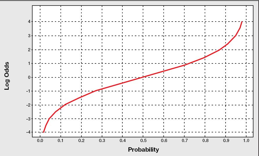
5 odds와 logit #
승산(그림 출처 ->
여기(http://www.bisolutions.us/Credit-Risk-Evaluation-of-Online-Personal-Loan-Applicants-A-Data-Mining-Approach.php))

로짓(그림 출처 ->
여기(http://www.bisolutions.us/Credit-Risk-Evaluation-of-Online-Personal-Loan-Applicants-A-Data-Mining-Approach.php)) = log와 odds를 합친말 = log(1/(1-p))
pred <- predict(german.object, german, type="response")
logodds <- predict(german.object, german)
german <- cbind(german, pred) #확률
german <- cbind(german, logodds) #오즈, odds
head(german)
결과
> head(german)
   x1 x2  x3 x4 x5 x6 y       pred    logodds
1 A11  6 A34  4 67  1 0 0.18091034 -1.5101920
2 A12 48 A32  2 22  1 1 0.63503244  0.5538676
3 A14 12 A34  3 49  2 0 0.04865313 -2.9731627
4 A11 42 A32  4 45  2 0 0.64246423  0.5860757
5 A11 24 A33  4 53  2 1 0.46964395 -0.1215737
6 A14 36 A32  4 35  2 0 0.19922819 -1.3911252
2번째 Row는
| x1 | x2 | x3 | x4 | x5 | x6 | y |
| A12 | 48 | A32 | 2 | 22 | 1 | 1 |
이고, 회귀식이 다음과 같으므로
Coefficients:
             Estimate Std. Error z value Pr(>|z|)
(Intercept)  0.665099   0.476311   1.396 0.162607
x1A12       -0.531864   0.185402  -2.869 0.004121 **
x1A13       -1.076082   0.336956  -3.194 0.001405 **
x1A14       -1.898800   0.206314  -9.203  < 2e-16 ***
x2           0.034342   0.006329   5.426 5.76e-08 ***
x3A31       -0.099153   0.474942  -0.209 0.834629
x3A32       -0.946961   0.370644  -2.555 0.010622 *
x3A33       -0.934327   0.433303  -2.156 0.031061 *
x3A34       -1.526069   0.393754  -3.876 0.000106 ***
x5          -0.012765   0.007091  -1.800 0.071821 .
다음과 같이 계산된다.
0.665099 -0.531864 + 48 * 0.034342 - 0.946961 -0.012765 * 22 = 0.5538676
확률은..
x <- 0.665099 -0.531864 + 48 * 0.034342 - 0.946961 -0.012765 * 22
1 / (1 + exp(-x)) #결과값 0.6350307
exp(x) / (1 + exp(x)) #결과값 0.6350307, 이게 로지스틱 모형
과 같이 계산하면 된다.
8 분류표(confusion matrix) #
#T1 <- length(german[german$y==1 & german$pred > 0.5,]$x1)
#T0 <- length(german[german$y==0 & german$pred > 0.5,]$x1)
#F1 <- length(german[german$y==1 & german$pred <= 0.5,]$x1)
#F0 <- length(german[german$y==0 & german$pred <= 0.5,]$x1)
#
install.packages("SDMTools")
library("SDMTools")
confusion.matrix(german$y,german$pred,threshold=0.5)
결과
> confusion.matrix(german$y,german$pred,threshold=0.5)
    obs
pred   0   1
   0 629 177
   1  71 123
attr(,"class")
[1] "confusion.matrix"
| | False(실제) | True(실제) |
| False(예측) | 629 | 177 |
| True(예측) | 71 | 123 |
| 항목 | 계산 | 확률(%) |
| 정확도 (Accuracy) | (629 + 123) / (629 + 177 + 71 + 123) | 75.20% |
| 민감도 (sensitivity) | 123 / (177 + 123) | 41.00% |
| 특이도 (specificity) | 629 / (629 + 71) | 89.86% |
| 오류율 (error) | (177 + 71 ) / (629 + 177 + 71 + 123) | 24.80% |
다음과 같이 R로 계산해도 된다.
library("SDMTools")
mat <- confusion.matrix(german$y,german$pred,threshold=0.5)
mat
omission(mat)
sensitivity(mat)
specificity(mat)
prop.correct(mat)
결과
> mat
    obs
pred   0   1
   0 629 177
   1  71 123
attr(,"class")
[1] "confusion.matrix"
> omission(mat)
[1] 0.59
> sensitivity(mat)
[1] 0.41
> specificity(mat)
[1] 0.8985714
> prop.correct(mat)
[1] 0.752
>
다음과 같이 하면 다 나온다.
> accuracy(german$y,german$pred,threshold=0.5)
  threshold       AUC omission.rate sensitivity specificity prop.correct     Kappa
1       0.5 0.6542857          0.59        0.41   0.8985714        0.752 0.3432203
>
값에 대한 설명
- AUC(area under curve): ROC curve 아래의 면적, 숫자가 높을수록 좋다.
- omission.rate: the ommission rate as a proportion of true occurrences misidentified given the defined threshold value
- sensitivity: 1일 확률, 민감도
- specificity: 0일 확률, 특이도
- prop.correct: 모델의 정확도
- kappa statistic
- Fleiss의 판단기준..
- 신뢰도 낮다: 0.4 미만
- 신뢰도 있다: 0.4 ~ 0.6
- 신뢰도 높다: 0.6 ~ 0.75
- 신뢰도 매우 높다: 0.75 초과
참고: 최적(정확도)의 threshold 찾기
for (i in seq(0,1,0.01))
{
  rs <- c(rs, accuracy(x2$t0,x2$pred,threshold=i)$prop.correct)
}

max_val = max(rs)
for (i in seq(0,1,0.01))
{
  tmp <- accuracy(x2$t0,x2$pred,threshold=i)$prop.correct
  if ( max_val == tmp )
  {
    print (paste("threshold = ", i))
  }
}
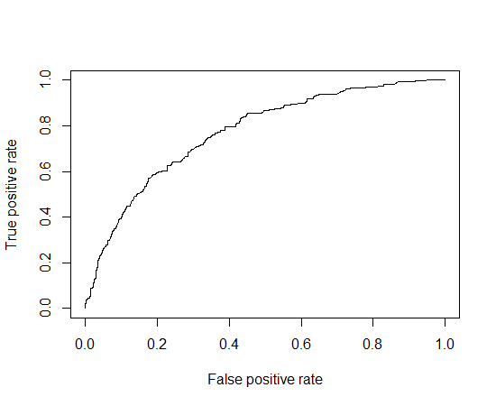
9 ROC(Receiver-Operating Characteristic curve) 곡선 #
install.packages("ROCR")
library("ROCR")
cname <- c("x1", "x2", "x3","x4", "x5", "x6", "y")
german = read.table("c:\\data\\german1.txt", col.names = cname)
options(contrasts = c("contr.treatment", "contr.poly"))
german.object <- glm(formula = y ~ x1 + x2 + x3 + x5, family = binomial, data = german)

pred <- predict(german.object, german, type="response")
logodds <- predict(german.object, german)
german <- cbind(german, pred)
german <- cbind(german, logodds)

roc = prediction(german$pred, german$y)
perf = performance(roc, "tpr", "fpr")
#"tpr"은 hit rate, "fpr"은 헛경보율(false alarm rate)
plot(perf)
#plot(perf, print.cutoff.at=seq(0,1,by=0.1))
install.packages("logistf")
library("logistf")
lr2 = logistf(y ~ x1 + x2 + x3 + x5, data = german)
summary(lr2)
결과
> summary(lr2)
logistf(formula = y ~ x1 + x2 + x3 + x5, data = german)

Model fitted by Penalized ML
Confidence intervals and p-values by Profile Likelihood

                   coef    se(coef)  lower 0.95   upper 0.95       Chisq
(Intercept)  0.64472876 0.474759083 -0.27043182  1.581359116  1.89900357
x1A12       -0.52660853 0.185120846 -0.88988344 -0.166823398  8.25198090
x1A13       -1.04548754 0.334474867 -1.72559520 -0.417128337 11.03319913
x1A14       -1.87794257 0.205266409 -2.28709164 -1.483111213         Inf
x2           0.03387929 0.006308928  0.02165981  0.046313848 29.94733537
x3A31       -0.09194231 0.473477203 -1.01911361  0.824239056  0.03855106
x3A32       -0.92696865 0.369386547 -1.66277580 -0.221680910  6.67102543
x3A33       -0.90779881 0.431809628 -1.76384501 -0.081117723  4.64170188
x3A34       -1.49870282 0.392307541 -2.27839153 -0.748208241 15.50420478
x5          -0.01252255 0.007063063 -0.02651766  0.001115517  3.23324577
                       p
(Intercept) 1.681899e-01
x1A12       4.070755e-03
x1A13       8.949457e-04
x1A14       0.000000e+00
x2          4.439416e-08
x3A31       8.443407e-01
x3A32       9.799279e-03
x3A33       3.120404e-02
x3A34       8.232193e-05
x5          7.215754e-02

Likelihood ratio test=200.5529 on 9 df, p=0, n=1000
Wald test = 152.8214 on 9 df, p = 0

Covariance-Matrix:
              [,1]          [,2]          [,3]          [,4]          [,5]
 [1,]  0.225396187 -2.116841e-02 -0.0178520944 -1.475598e-02 -1.030299e-03
 [2,] -0.021168410  3.426973e-02  0.0158947775  1.663656e-02 -4.993463e-05
 [3,] -0.017852094  1.589478e-02  0.1118734364  1.582290e-02  1.008258e-04
 [4,] -0.014755985  1.663656e-02  0.0158228986  4.213430e-02 -6.926150e-05
 [5,] -0.001030299 -4.993463e-05  0.0001008258 -6.926150e-05  3.980257e-05
 [6,] -0.129133562  4.653294e-03  0.0017777035  2.271459e-03  1.822720e-04
 [7,] -0.134642541  3.932850e-03  0.0010335670  1.458292e-04  2.134383e-04
 [8,] -0.118628622 -2.470301e-03  0.0005935660 -5.484439e-03 -2.417103e-05
 [9,] -0.126861265  4.418244e-03  0.0018526164 -2.134237e-03  2.052452e-04
[10,] -0.001743630  7.292805e-05 -0.0000437410  1.938701e-05 -1.300694e-07
               [,6]          [,7]          [,8]          [,9]         [,10]
 [1,] -1.291336e-01 -1.346425e-01 -1.186286e-01 -0.1268612649 -1.743630e-03
 [2,]  4.653294e-03  3.932850e-03 -2.470301e-03  0.0044182436  7.292805e-05
 [3,]  1.777704e-03  1.033567e-03  5.935660e-04  0.0018526164 -4.374100e-05
 [4,]  2.271459e-03  1.458292e-04 -5.484439e-03 -0.0021342366  1.938701e-05
 [5,]  1.822720e-04  2.134383e-04 -2.417103e-05  0.0002052452 -1.300694e-07
 [6,]  2.241807e-01  1.258971e-01  1.240776e-01  0.1263132224 -8.388392e-05
 [7,]  1.258971e-01  1.364464e-01  1.240557e-01  0.1260949748  7.408724e-05
 [8,]  1.240776e-01  1.240557e-01  1.864596e-01  0.1247551153 -9.031551e-05
 [9,]  1.263132e-01  1.260950e-01  1.247551e-01  0.1539052064 -1.431441e-04
[10,] -8.388392e-05  7.408724e-05 -9.031551e-05 -0.0001431441  4.988686e-05
이런거도 있다.
install.packages("survey")
library("survey")
regTermTest(german.object, ~x1 + x2 + x3 + x5)
결과
> regTermTest(german.object, ~x1 + x2 + x3 + x5)
Wald test for x1 x2 x3 x5
 in glm(formula = y ~ x1 + x2 + x3 + x5, family = binomial, data = german)
F =  17.2046  on  9  and  990  df: p= < 2.22e-16
p-value가 조넨 작으니까 귀무가설 지지 못함. 즉, 차이가 있음.
 german1.txt) 활용
![[-]](/moniwiki/imgs/plugin/arrup.png "[-]")
![[+]](/moniwiki/imgs/plugin/arrdown.png "[+]")